Dijkstra's Algorithm: The Ultimate Guide 2025
Introduction
In the realm of computer science and graph theory, Dijkstra’s Algorithm is one of the most widely used methods for finding the shortest path between nodes in a weighted graph. Developed by Edsger W. Dijkstra in 1956 and published in 1959, the algorithm remains an essential tool for solving real-world shortest path problems efficiently.
From GPS navigation to network routing, logistics, and artificial intelligence, Dijkstra’s Algorithm plays a crucial role in optimizing paths and minimizing travel or communication costs. In this blog, we will explore its working principles, implementation, optimizations, real-world applications, and a comparative analysis with other shortest path algorithms.
Understanding Dijkstra’s Algorithm
What is Dijkstra’s Algorithm?
Dijkstra’s Algorithm is a graph traversal algorithm used to compute the shortest path between a starting node and all other nodes in a weighted graph. It operates by selecting the nearest unvisited node, updating distances to its neighbors, and repeating the process until all nodes are processed.
Key Characteristics:
Greedy Strategy: Always selects the closest unvisited node to process next.
Graph Compatibility: Works on directed and undirected graphs but requires non-negative edge weights.
Guaranteed Optimality: Always finds the shortest path from the source to all reachable nodes.
Efficiency: Performs well for small to medium-sized graphs, but requires optimizations for very large graphs.
How Does It Differ from Other Algorithms?
Unlike Bellman-Ford, which works with negative weights but has a higher time complexity, Dijkstra’s Algorithm is more efficient and widely preferred when all edge weights are non-negative.
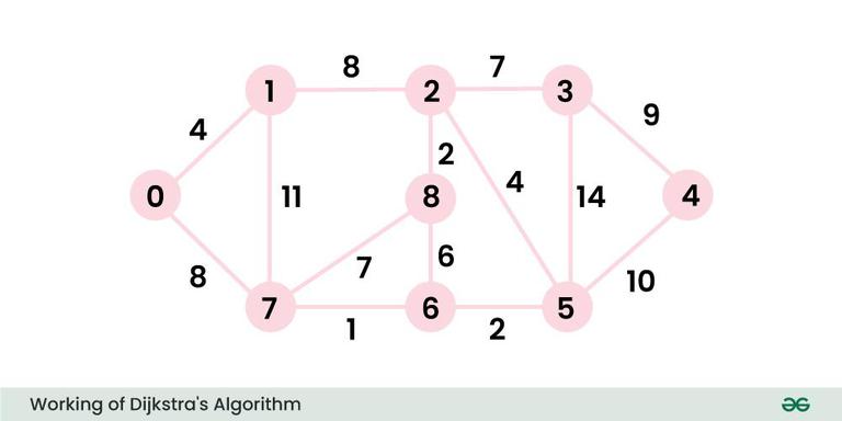
Step-by-Step Explanation
Dijkstra’s Algorithm follows a systematic approach to finding the shortest path in a graph:
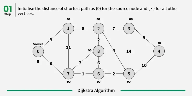
Initialization:
Assign 0 as the starting node’s distance and infinity for all others.
Store all nodes in a priority queue (min-heap) with their respective distances.
Priority Queue Operations:
Extract the node with the smallest distance from the queue.
If this node has been processed before, skip it.
Relaxation Step:
For each unvisited neighbor of the current node:
Calculate a new distance by adding the edge weight to the current node’s distance.
If the new distance is shorter than the recorded distance, update it.
Insert the updated node into the priority queue.
Mark Node as Processed:
Mark the current node as visited so it is not processed again.
Repeat Until Completion:
Continue the process until all nodes are processed or until the shortest path to a specific node is found.
Resources
- [Dijkstra’s Algorithm Code on GitHub](https://gist.github.com/MagallanesFito/61afb009986f0319774cb079b8914bb2)
- Related algorithms: Bellman-Ford, A* Search
Here’s a line-by-line explanation of the code:
#include <bits/stdc++.h>: Includes all standard C++ libraries (like vectors, lists, queues, etc.).-
#define INF 0x3f3f3f3f: Defines a large integer (1061109567), used as infinity (INF) in shortest path calculations. -
using namespace std;: Avoids usingstd::before standard library functions.
- Defines
myPairaspair<int, int>to represent edges as{vertex, weight}.
Graphclass represents a weighted graph.-
int V: Number of vertices. -
list<myPair> *adj: An adjacency list where each vertex stores a list of{neighbor, weight}. -
Graph(int V): Constructor to initialize the graph. -
void addEdge(int u, int v, int w): Adds an edge between verticesuandvwith weightw. -
void shortestPath(int src): Implements Dijkstra’s algorithm.
Initializes
Vwith the given number of vertices.-
Dynamically allocates an array of adjacency lists (
adj).
Adds an edge
{v, w}tou’s adjacency list.-
Adds
{u, w}tov’s adjacency list (since the graph is undirected).
- Implements Dijkstra’s algorithm to find the shortest path from
srcto all other vertices.
- Uses a min-heap (
priority_queue) to always process the vertex with the smallest distance first.
- Initializes a distance vector (
dist) of sizeVwithINF.
- Distance to the source vertex is
0.
- Iterator to traverse adjacency lists.
- Pushes
{0, src}into the priority queue (source with distance0).
- Runs until all vertices are processed.
- Extracts the vertex
uwith the smallest distance.
- Iterates over all neighbors (
v) ofuand their corresponding weights (w).
- If a shorter path to
vis found, updatedist[v]and push{dist[v], v}into the queue.
- Prints the shortest distance from
srcto each vertex.
- Creates a graph with
5vertices.
- Calls
shortestPath(0)to compute shortest paths from vertex0.
Time Complexity Analysis
The efficiency of Dijkstra’s Algorithm depends on the data structures used:
Using a Simple Array: O(V²) (Less efficient for large graphs)
Using a Binary Heap (Priority Queue): O(V log V + E log V) (More efficient for sparse graphs)
Using a Fibonacci Heap: O(E + V log V) (Optimal for large graphs)
Optimizations
To improve performance, consider the following optimizations:
Fibonacci Heap: Reduces priority queue operations, making the algorithm more efficient for large graphs.
Bidirectional Dijkstra: Runs two simultaneous searches—one from the start node and one from the destination—reducing the number of processed nodes.
A Algorithm*: Uses heuristics (such as Euclidean distance) to prioritize paths that are more likely to reach the goal faster.
Graph Pruning: Removes unnecessary nodes or edges before execution to enhance performance.
Real-World Applications
Dijkstra’s Algorithm is widely used in various industries:
Navigation Systems: GPS applications like Google Maps and Waze use it to determine the shortest driving or walking routes.
Network Routing: Internet routers implement Dijkstra’s Algorithm to find the best data transmission path.
Game AI Pathfinding: Video games use it to calculate the optimal movement of AI characters on maps.
Logistics & Transportation: Delivery companies like FedEx and UPS use it to optimize shipment routes.
Robotics: Autonomous robots use it for obstacle avoidance and movement planning.
Limitations of Dijkstra’s Algorithm
While Dijkstra’s Algorithm is highly efficient, it has some limitations: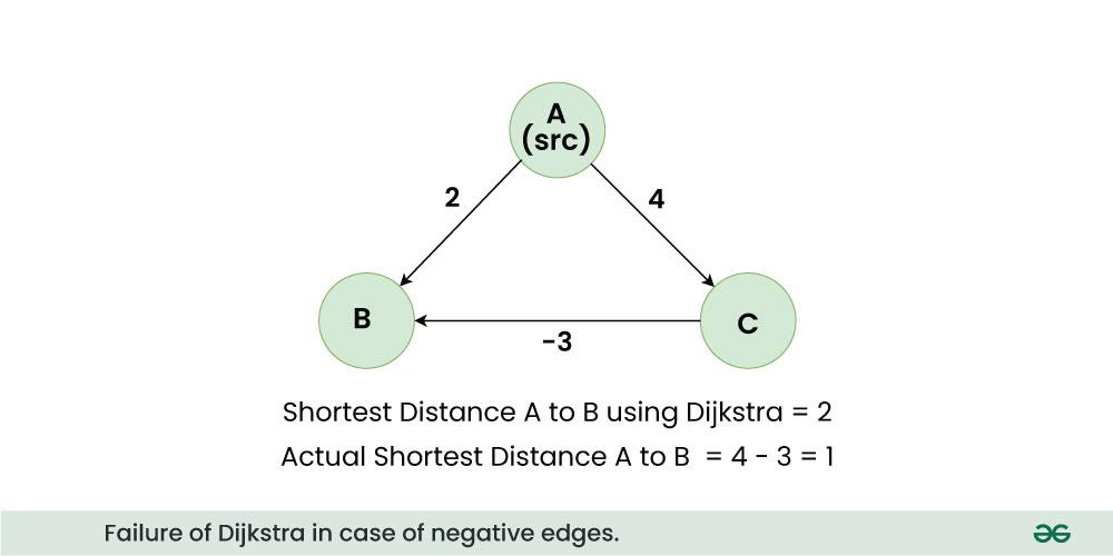
Cannot Handle Negative Edge Weights: The presence of negative weights can cause incorrect results, unlike the Bellman-Ford Algorithm.
- Inefficient for Large Graphs: For graphs with millions of nodes, optimizations are necessary to improve performance.
- Not Ideal for Dynamic Graphs: If the graph changes frequently (e.g., real-time traffic updates), re-running the algorithm can be computationally expensive.
Conclusion
Dijkstra’s Algorithm remains a cornerstone of graph theory and shortest path computations. It is widely used in navigation, networking, logistics, robotics, and artificial intelligence. Despite its limitations, optimizations like Fibonacci heaps, bidirectional search, and heuristic-based methods make it a powerful tool for modern computing challenges.
Understanding Dijkstra’s Algorithm and its variations will enhance your problem-solving skills, making it a valuable asset for software engineers, AI researchers, and data scientists. Keep exploring new optimizations and real-world applications to master its potential!
Comments
Post a Comment